Specifying the estimation type (page 2/5)

1. Click on nonlinear at the bottom of the equations window.
2. Choose 2nd order PQL -for technical reasons this gives better estimates of the variance components than the default.

   

   An aside: Using MCMC estimation instead - some research shows that PQL variance estimates, whilst better than MQL estimates (the default in MLwiN) as still downwardly biased i.e. underestimate the extent of variation. Once we have estimated the parameters in MLwiN using PQL we can switch to Monte Carlo Markov Chain estimation by clicking on the 'estimation control' window and choosing 'MCMC'. Then re-estimate the model parameters using the PQL estimates as 'starting values' in the iterative process. We illustrate this below for this model. We could use this approach for any of the multilevel models. For more details see references on www.cmm.bristol.ac.uk
3. Now click on 'start' in the top left of the programme window. The parameters will turn from blue to green when the estimation process has converged.
4. Click on the Estimates button at the bottom of the equations screen to see the estimated values:

   

   The mean is 1.643 (on the logit scale). To convert back from logit to probability use

   e^1.643 / (1+ e^1.643) = 0.838

   where 'e' is the exponential function.

   So the overall proportion reporting that they turned out to vote in this sample is 0.838 (this represents an average turnout of nearly 84%). We know that in the actual elections a lower proportion turned out. Hence some people are reporting in the ESS that they turned out to vote in the most recent election when in fact they did not (and/or the sampling process has lead to an oversampling of voters). We can account for this partially by using weights. See, for example, the post-stratification approach as used by Fieldhouse, Tranmer and Russell (2007). ). For now we will continue with the figures as they are.

   The country level variation is estimated as 0.299 on the logit scale, suggesting there is considerable variation between countries with respect to voter turnout.

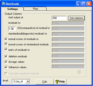
   We can save and plot the country level residuals from this model. Choose 'residuals' from the model menu.

   

   

   

   And set the comparative s.d. as 1.96 and the level to be 2:ctry_id.

5. Also -click on 'set columns'.
6. Now click on plots and choose 'residual' +/- 1.96 s.d x rank and click 'apply'.

   

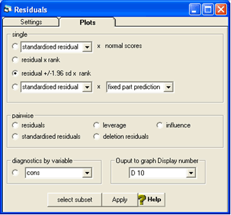
   We get this 'caterpillar' plot. The residuals Uoj are plotted in ascending order of magnitude with their confidence intervals. Where this confidence interval crosses the 0.0 line the turnout for that country is not significantly different from the overall turnout in Europe. If the confidence interval is entirely below the dotted line the turnout is significantly lower for that country and if the confidence interval is entirely above the dotted line the turnout is significantly higher for that country. The plot is interactive -we can click on a residual to find out the country id. For example the first residual on the plot is country id 19 (Poland) and the last one is country id 11 (Greece).